Artificial Intelligence

Chapter 3: Artificial Intelligence

1. Introduction to artificial intelligence
2. Overview of techniques used in artificial intelligence
3. Artificial neural networks
4. Deep learning networks and computer vision technique
5. Challenges and solutions in the training process

3.1 Introduction to Artificial Intelligence

3.1.1 Introduction

For a long time, humans have tried to understand how thinking works — including the perception and interpretation of reality as well as the prediction and processing of information. Artificial intelligence refers to the imitation of human intelligence in machines that are programmed to think like humans and especially to learn and solve problems. Serious research began after World War II; the current designation was established in 1956. For researchers, the possibilities remain open.

3.1.2 Concept (Russell & Norvig, 2002a)

Definitions of artificial intelligence differ depending on researchers and disciplines. The focus is on thought and reasoning processes as opposed to behavior on the one hand, and human performance as opposed to ideal performance on the other. From the combination of these axes, four studied concepts emerge:

• Human performance: embodied by the Turing test developed by Alan Turing in 1950. A machine is considered intelligent if it can answer questions from a human examiner without the examiner being able to determine whether the answer comes from a human or a machine.
• Human thinking: an example is the General Problem Solver of Newell and Simon (1961). The researchers attempted to use the same steps that humans use to solve problems, regardless of how accurate the result is.
• Rational thinking: it is based on Aristotle's ideas for developing correct rules for thinking and reasoning, i.e., logic. If Ahmad is taller than Mohammad and Mohammad is taller than Said, it follows that Ahmad is taller than Said.
• Rational action: the goal is the best possible expected outcome. This includes logical thinking through reasoning. However, in some situations there is no clearly correct action; one option may only probably be better than another. Also reflex actions, such as withdrawing the hand after touching a hot surface, can be the best option without waiting for detailed reasoning.

3.1.3 Historical Overview (Mijwel, 2015; Russell & Norvig, 2002a)

Warren McCulloch and Walter Pitts developed the first model of artificial neurons. It responded when sufficient stimulation arrived from the connected surrounding neurons. The basis was physiological findings about neurons, logical analysis, and Turing's computation theory, such as for building logical gates (NOT, OR, AND). Further research followed. The era was shaped by Turing's proposals: the Turing test and the idea of imitating the learning mind of a child rather than the thinking patterns of an adult.

John McCarthy founded the discipline by gathering ten scientists for two months at Dartmouth University in Hanover in 1956. An important result was the Logic Theorist (LT) by Allen Newell and Herbert Simon. It enabled computers to think logically rather than only numerically and to solve problems, and established a research community that continued to develop the field in subsequent years.

This was followed by a golden age with numerous AI applications demonstrating that computers could perform more than arithmetic operations: the General Problem Solver (Newell and Simon), a system for proving geometric theorems (Herbert Gelernter, 1959), and a chess program (Arthur Samuel) whose performance could improve and eventually beat the developer. McCarthy developed the programming language LISP, which was used as an AI language for a long time. At the same time, limited resources and the weak performance of computers at that time constrained research.

In the late 1960s and early 1970s, it became apparent that the excessive optimism of some researchers had overestimated the capabilities of AI. This was based on experiments in a limited environment that were not transferable to reality. Tasks such as machine translation, which had been supported by the US government, also proved to be of limited success; support was withdrawn. The widespread assumption that the limits of AI at that time were solely due to limited computing power was also inaccurate.

A phase of stagnation ensued, including for artificial neural networks. Earlier research had focused on general intelligent systems that achieved virtually no good results; their significance was limited to a few games and simple tasks, and government support declined. Subsequently, attention turned to systems for solving specific problems. The first expert system was DENDRAL. It was designed to analyze the composition of Mars soil based on spectroscopic signals. For this, experts were involved and rule-based knowledge bases were created. Numerous expert systems emerged during this period; programming languages and computer technology developed in parallel.

By the late 1980s, the conditions were in place for the return of artificial neural networks. Lessons were learned from past experiences, the focus was placed on specific tasks, and developments in programming languages and computers were leveraged. Above all, advances in learning algorithms, particularly backpropagation, led to a powerful resurgence of artificial neural networks in many application areas.

3.2 Overview of Artificial Intelligence Techniques

AI techniques developed in parallel with our understanding of artificial intelligence. The most important include:

3.2.1 Search Algorithms

Search algorithms are among the earliest techniques. They attempt to examine all possible moves, as in chess. Initially, the search was blind and undirected, which burdened the speed and complexity of the task. Later, heuristic search methods were developed that made the algorithms more efficient. A well-known example is Samuel's checkers program (Jones, 2008).

3.2.2 Expert Systems

The basic idea is to transfer the knowledge of a human expert on a particular topic to a computer. A knowledge engineer accomplishes this by documenting information as rules. Through a prepared user interface, the user then receives a recommendation and an explanation based on the entered data (Liao, 2005).

DENDRAL is one of the most well-known expert systems. It was used for chemical analysis of Mars soil to determine the molecular structure from spectroscopic signals. The rules needed for this were created by experts, since shipping conventional analytical equipment was not feasible (Feigenbaum & Buchanan, 1994). Expert systems, unlike humans, provide fixed outputs without creativity. Errors in knowledge transfer lead to incorrect results. Additionally, development and modification when extending or adapting rules are costly (Cowan, 2001; Partridge, 1987).

3.2.3 Machine Learning

Machine learning can be simply described as learning from examples. It includes (Bonaccorso, 2017; Jatana, 2019):

• Supervised learning: there is a reference for what is right and wrong; performance is improved by reducing error. Regression algorithms have continuous numerical outputs, such as blood pressure or weight. Examples include linear regression, support vector machine (SVM), decision tree, random forest, boosting, and neural networks. Classification algorithms produce a specific class, such as assigning an image to one of three classes. Examples include logistic regression, naive Bayes, SVM, decision tree, random forest, boosting, and neural networks.
• Unsupervised learning: there is no reference; relationships within the data are extracted and grouped by similarity. A well-known algorithm is K-means.
• Reinforcement learning: there is neither teacher nor reference. The learning process during training is controlled through a reward and punishment system. This is important in a continuously changing, not fully predictable environment, such as video games with a long-term strategic goal and short-term subgoals. Reinforcement learning can make immediate rational decisions and accept a short-term loss in favor of a long-term gain.

3.2.4 Evolutionary and Genetic Algorithms

These algorithms are based on fundamental principles of biology, evolutionary theory, natural selection, spontaneous mutation, and survival of the fittest. Suitable traits for solving a problem are found by allowing generations with unfavorable traits to die out and generations with favorable traits to be preserved and reinforced through crossover and random exchange of these traits in producing the next generation. A low rate of random mutations can produce new, previously nonexistent traits that aid in problem-solving (Coello, 2005; Yu & Gen, 2010).

3.3 Artificial Neural Networks

3.3.1 Concept

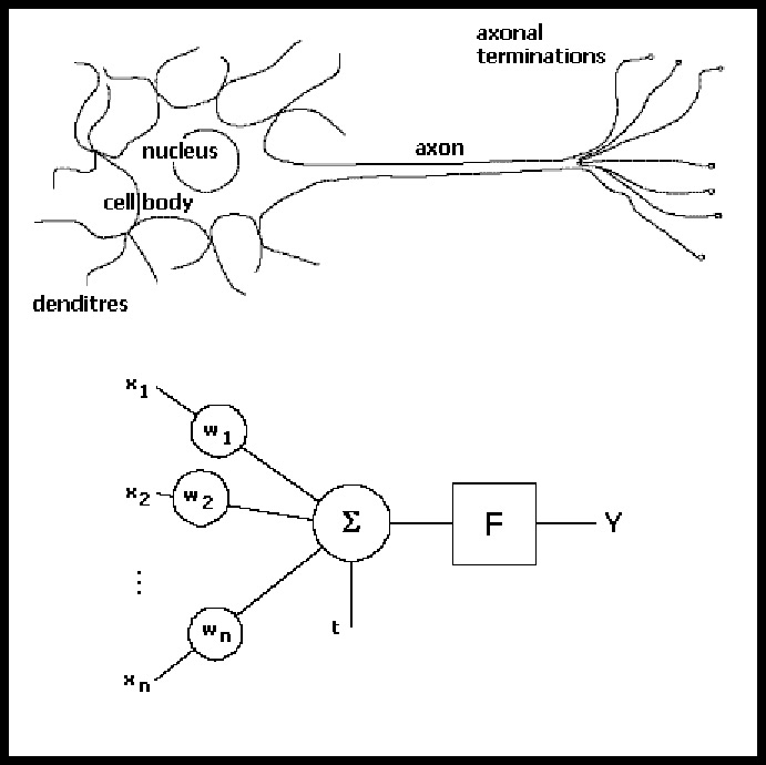
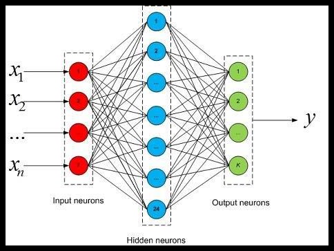
The idea of artificial neural networks is inspired by biological nerve cells and their connections in the brain (Figure 25). Each neuron consists of inputs, a function, and an output; this corresponds to the dendrites, the cell body, and the axon. In a neural network, neurons are connected in successive layers. The simplest structure consists of an input layer, a hidden layer, and an output layer (Figure 26). Each neuron is connected to all neurons in the previous and subsequent layers (Scarborough & Somers, 2006).

3.3.2 Training

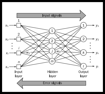
The network is trained with a database containing inputs and outputs. The data are split into training, validation, and test groups. Inputs from the training group are fed into the network; the output is calculated, compared with the actual value, and the connections within the network are adjusted to reduce the error. The error is called the loss (Figure 27). Training is repeated multiple times; in each run, accuracy is calculated on the validation group.

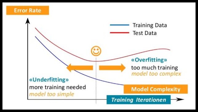
Typically, accuracy in both the training and validation groups initially rises (learning process). At a certain point, the groups diverge: training accuracy continues to rise while validation accuracy declines. This is overfitting. Learning then effectively ends in memorizing the training group, which degrades performance on the validation group (Figure 28). Subsequently, accuracy is calculated on an independent test group; this represents the expected result of the model when applied in practice (Smola & Vishwanathan, 2008).

3.3.3 Advantages and Disadvantages of Artificial Neural Networks

Advantages: Neural networks can model complex and nested relationships, nonparametric relationships, weak relationships between dependent and independent variables, as well as high unexplained variance. They are also usable when no clear theoretical basis for prediction or classification can be formulated (Scarborough & Somers, 2006; Sarle, 1994). Additional properties include:

• no fixed restriction on the type of inputs and outputs; qualitative and quantitative variables and mixed forms are possible;
• no prior assumptions about the statistical distribution of variables or their relationships;
• no fixed number of inputs and outputs;
• high computational efficiency and therefore real-time analysis;
• a dynamic, flexible nonlinear regression system (Niavarani & Wickramasinghe, 2014).

Disadvantages (Hastie, Tibshirani, & Friedman, 2001): A good model requires good training with sufficiently large and high-quality data. It is difficult to recognize what exactly is happening in the model (black box); essentially, only inputs and outputs are visible.

3.4 Deep Learning and Computer Vision

3.4.1 Deep Learning

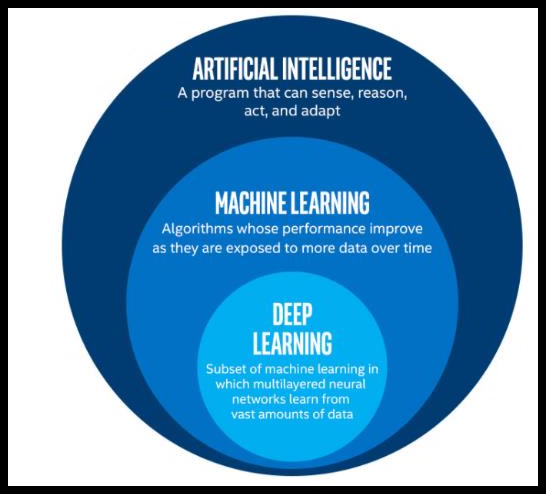
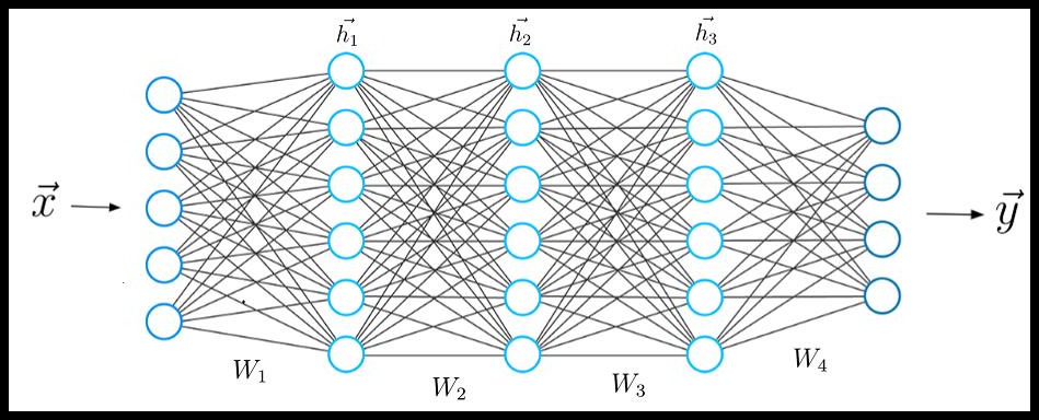
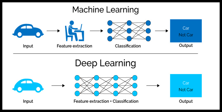
Deep learning is a subfield of machine learning (Figure 29) and initially emerged in 2006. It is primarily used for pattern recognition. A network consists of multiple hierarchically arranged neuron layers (Figure 30). The goal is to extract useful information and features. This distinguishes deep learning from conventional machine learning methods, where the useful features are predetermined before classification and extracted with independent techniques outside the neural network. Deep learning can be supervised or unsupervised (Figure 31; Vargas, Mosavi, & Ruiz, 2017).

3.3.2 Computer Vision and Convolutional Neural Networks

Computer vision is a subfield of artificial intelligence. Computer vision algorithms aim to develop intelligent applications that can understand the content of images like humans. One of the most common techniques for this are convolutional neural networks (CNN). They are multilayered artificial neural networks and therefore belong to deep learning. CNN can take images as inputs and, through multiple neuron layers that act like filters, extract information. The dimensions are progressively reduced until a one-dimensional neuron matrix is produced, which is connected with additional layers. The last layer contains as many neurons as the classes to be recognized. Due to the reduced number of connections to be determined compared to conventional neural networks, the probability of overfitting is reduced (O'Shea & Nash, 2015).

Convolutional Layer: It takes an input image with length, width, and depth and scans it with several matrices. Each matrix consists of multiple neurons and is moved over the entire image by multiplication with the corresponding image section. The result is displayed as a number matrix; subsequently, in the activation layer, an activation function is applied, producing several feature maps — one for each neuron matrix (Figures 32–33). The matrices act like filters and extract important features (Jeong, 2019).

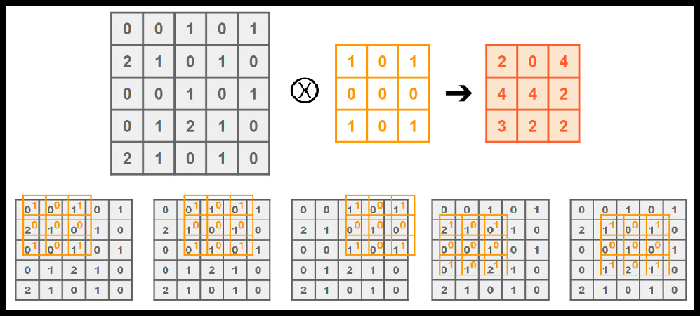
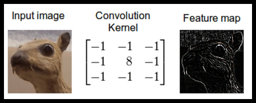
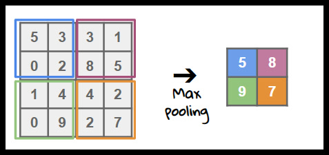
Pooling Layer: It progressively reduces the dimensions of the outputs of the convolutional layer without changing the depth. In the commonly used max pooling, a neuron matrix, for example 2×2, scans the image and selects only the highest value; the remaining values are discarded. In this example, the image size is reduced to one quarter (Figure 34; Jeong, 2019).

Activation Layer (Rectified Linear Units Layer): It consists of neurons that apply an activation function to the output of each neuron of the convolutional layer. The resulting feature map highlights important features and suppresses unimportant ones. A key objective is to accelerate training: the output of each neuron depends only on its input and not on the values of other neurons (Figure 33; Jeong, 2019).

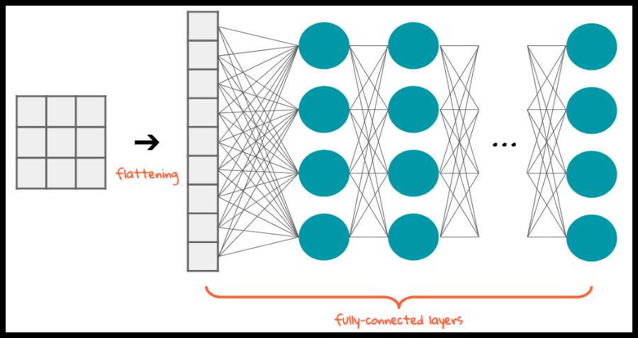
Flattening Layer: Input matrices are converted into a one-dimensional vector. This neuron vector forms the input layer of a conventional multilayered artificial neural network that ends in an output layer with as many neurons as trained classes (Figure 35; Jeong, 2019).

Fully Connected Layers and Output Layer: Multiple layers end in an output layer with one neuron per trained class and an appropriate activation function (Figure 35; Jeong, 2019).

3.5 Challenges and Solutions in the Training Process

During training, problems and challenges arise that affect model accuracy. Some, such as overfitting, are general; others occur more frequently in the medical field, particularly imbalanced classes and small sample sizes. The most important problems and possible solutions are summarized below.

3.5.1 Overfitting

The problem has already been explained in the section on training. Possible techniques include:

• Cross-Validation: The training group is divided into, for example, five parts. Four parts are used for training and the fifth for testing. The process is repeated five times; each portion serves once as the test group. Population accuracy can be estimated by the mean of the five test accuracies (Moore, 2001).
• Regularization: The model is penalized during training to make it simpler to a certain degree (Russell & Norvig, 2002b). In L1, the penalty corresponds to the sum of the absolute values of the weights. Features with weights near zero are removed; the model becomes more interpretable and the number of features used decreases. L2 is more common and penalizes with the sum of the squared weights. The weights approach zero but do not reach zero.
• Early Stopping: Training is terminated when training and validation accuracy diverge, so that both accuracies are still similar (Sarle, 1996).
• Dropout: Connections between some neurons of a layer and the following layer are randomly removed with a certain probability. This reduces overfitting (Srivastava, Hinton, Krizhevsky, Sutskever, & Salakhutdinov, 2014).

3.5.2 Small Dataset

This problem is common in medicine because databases with millions of data records are rare, especially for medical images. Data volumes usually comprise hundreds or thousands of cases. This can lead to underfitting, as the trained model does not achieve good results in the population. Solutions include (Han, Liu, & Fan, 2018):

• Transfer Learning: Training a network that has already been trained on a similar task is easier than training from scratch. Like a child who already knows numbers and addition, a pre-trained network needs less data and less time.
• Data Augmentation: The image is slightly modified, for example by rotating by a certain angle, horizontal or vertical flipping, or adding small noise. This produces new images similar to the original sample. For corneal topography maps, horizontal flipping can generate new training images due to the symmetry about the vertical line.

3.5.3 Class Imbalance

This problem occurs frequently in medicine because disease cases are much rarer than normal findings. A model trained with 90% normal and 10% diseased cases can achieve 90% accuracy by classifying every case as normal. When applied to the population, this also leads to underfitting. Common solutions are sampling and weighted loss (Abd Elrahman, Abraham, & Computing, 2013; Buda, Maki, & Mazurowski, 2018).

In sampling, the classes are balanced: in over-sampling, the rarer class in the training group is enlarged by repeated copying. This can cause overfitting; SMOTE therefore generates similar but not identical cases. In under-sampling, cases of the more frequent class are deleted. This can cause underfitting; methods such as GSVM-RU remove unimportant and duplicate cases while preserving important cases.

In weighted loss, the training loss is weighted to create a balance between the classes. The loss of the rare class is increased, and the loss of the common class is decreased. For this, the class-specific loss is multiplied by weights that are inversely proportional to the proportion of the class among all cases in the training group.