Chapter 5 · complete English translation

Study Design and Methods

Chapter 5: Study Design and Methods

Study design
Study group
Sample size
Inclusion and exclusion criteria and technical image characteristics
Characteristics of the study groups
Study methods

5.1 Study Design

Part 1: retrospective review of records and topographic images of patients who underwent topographic examination in the Department of Ophthalmology and Ophthalmic Surgery at Al-Mouassat University Hospital, University of Damascus. The aim was to collect and classify as many images as possible, perform descriptive statistical analyses, and use the data for training the AI system.
Part 2: cross-sectional study to determine the performance of the AI system.

5.2 Study Group

Part 1 aimed to collect as many images as possible from old records for training the system and to perform descriptive statistical evaluation. Part 2 consisted of a random sample of patients who visited the outpatient ophthalmology clinic at Al-Mouassat University Hospital.

5.3 Sample Size

For Part 1, the required sample size for a descriptive study was calculated with G*Power 3.0.10 at alpha = 0.05, beta = 0.05, and an effect size of 0.05. For a power of 95%, 356 patients were required. For Part 2, at alpha = 0.05, beta = 0.05, an odds ratio of 2, and a proportion of discordant pairs of 0.3, a required sample of 380 eyes for a power of 95% was calculated with G*Power 3.0.10.

5.4 Inclusion and Exclusion Criteria and Technical Image Characteristics

Inclusion: age over 10 years; cooperation at the topography device for capturing a technically suitable image (Part 2) or presence of a previously captured technically suitable topographic image (Part 1).

Exclusion: lack of cooperation during image acquisition; previous images without technical suitability; children under 10 years of age; severe dry eye and ocular surface diseases; corneal dystrophies and degenerations; other ectatic corneal diseases; previous eye surgery, particularly on the cornea; corneal scarring from any cause other than keratoconus.

Technical image characteristics: The SIRIUS device software Phoenix v2.0.0.3 was used to assess technical suitability. The device evaluates coverage and proportion of unedited data (Not Edited) of the Scheimpflug camera as well as coverage and centration of the keratoscopy images. Based on this, it determines whether the image is technically suitable (CSO, 2018).

5.5 Characteristics of the Study Groups

5.5.1 Training Group

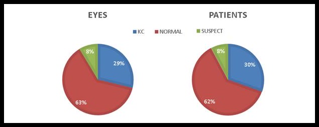
The training sample comprised 987 patients in three diagnostic groups (Figure 42): 300 keratoconic (KC; 30.39%), 610 normal (NORMAL; 61.80%), and 77 suspect (SUSPECT; 7.8%). At the eye level, it comprised 1,943 eyes: 559 KC (28.73%), 1,217 normal (62.67%), and 167 suspect eyes (8.6%).

Extracted original figure 42: Distribution of the Training Group by Diagnosis — **Figure 42.** Distribution of the Training Group by Diagnosis Source: Original dissertation, Original p. 100. Figure area extracted locally from the original PDF.

By sex, 483 were female (48.9%) and 504 were male (51.1%); the male-to-female ratio was 1.041753653. The chi-square test showed no statistically significant difference between males and females in the three groups (p > 5%; Table 6).

Table 6: F 483 (48.9%, cumulative 48.9%), M 504 (51.1%, cumulative 100.0%), Total 987 (100.0%).

Age ranged from 10 to 87 years, with a mean of 31.89 years. The Kolmogorov-Smirnov test yielded p = 0.000; age was not normally distributed and nonparametric tests were used (Tables 7–8).

Table 7: N = 987; Range 77.0; Minimum 10.0; Maximum 87.0; Mean 31.739; Standard deviation 13.1865; Valid N = 987.

Table 8: Kolmogorov-Smirnov 0.157, df 987, significance 0.000; Shapiro-Wilk 0.874, df 987, significance 0.000; Lilliefors significance correction.

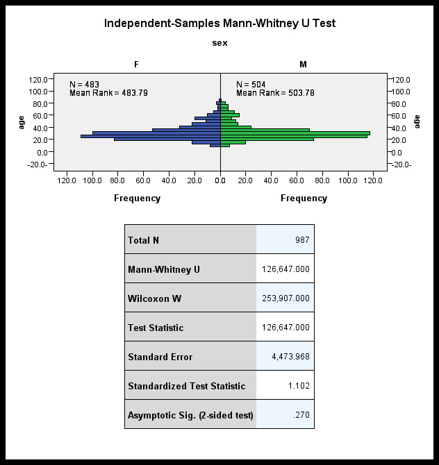
Mean age was 32.4 years for females and 31.37 years for males. The Mann-Whitney test showed no significant difference (p = 0.270; Figure 43).

Table 9: Females mean 31.20, 95% CI 30.08–32.33, median 28, SD 12.583, minimum 10, maximum 85; males mean 32.24, CI 31.04–33.44, median 29, SD 13.732, minimum 10, maximum 87.

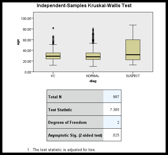
Extracted original figure 43: Mann–Whitney Test for Age Distribution by Gender in the Training Group — **Figure 43.** Mann–Whitney Test for Age Distribution by Gender in the Training Group Source: Original dissertation, Original p. 103. Figure area extracted locally from the original PDF.

By diagnosis, mean ages were KC 30.97 (12–82 years), NORMAL 31.03 (10–81 years), and SUSPECT 40.32 (13–87 years). The Kruskal-Wallis test showed a significant difference (p = 0.025; Table 10; Figure 44).

Table 10: KC mean 30.97, CI 29.71–32.22, median 29, SD 11.054, minimum 12, maximum 82; NORMAL 31.03, CI 30.03–32.02, median 28, SD 12.531, minimum 10, maximum 81; SUSPECT 40.32, CI 35.58–45.06, median 32, SD 20.875, minimum 13, maximum 87.

Extracted original figure 44: Kruskal–Wallis Test for Age Distribution by Diagnosis in the Training Group — **Figure 44.** Kruskal–Wallis Test for Age Distribution by Diagnosis in the Training Group Source: Original dissertation, Original p. 104. Figure area extracted locally from the original PDF.

5.5.2 Test Group

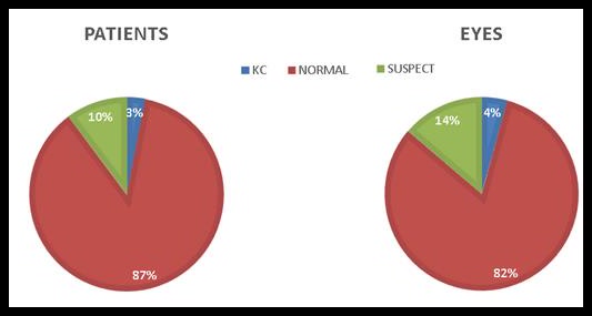
The test sample comprised 211 patients (Figure 45): 9 KC (4.27%), 173 normal (81.99%), and 29 suspect (13.74%). At the eye level, it comprised 422 eyes: 13 KC (3.08%), 366 normal (86.73%), and 43 suspect eyes (10.19%).

Extracted original figure 45: Distribution of the Test Group by Diagnosis — **Figure 45.** Distribution of the Test Group by Diagnosis Source: Original dissertation, Original p. 105. Figure area extracted locally from the original PDF.

By sex, the test group comprised 91 female (43.1%) and 120 male (56.9%) patients; the male-to-female ratio was 1:1.318. The chi-square test showed no significant difference between the three groups (p > 5%; Table 11).

Table 11: Distribution of the test group by sex and diagnosis with chi-square test.

Age ranged from 11 to 67 years, with a mean of 27.507 years (Table 12). The Kolmogorov-Smirnov test yielded p = 0.000; age was not normally distributed (Table 13).

Table 12: N = 422; Range 56.0; Minimum 11.0; Maximum 67.0; Mean 27.507; SD 12.4867; Valid N = 422.

Table 13: Kolmogorov-Smirnov 0.273, df 422, significance 0.000; Shapiro-Wilk 0.786, df 422, significance 0.000; Lilliefors correction.

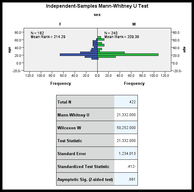
Mean age was 27.44 years for females and 27.55 years for males (Table 14). The Mann-Whitney test showed no significant difference (p = 0.681; Figure 46).

Table 14: Females mean 27.44, CI 25.69–29.18, median 23, SD 11.906, minimum 11, maximum 61; males mean 27.55, CI 25.91–29.20, median 23, SD 12.933, minimum 11, maximum 67.

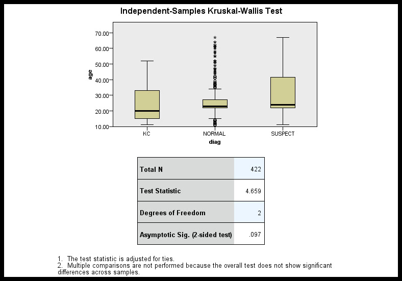
Extracted original figure 46: Mann–Whitney Test for Age Distribution by Gender in the Test Group — **Figure 46.** Mann–Whitney Test for Age Distribution by Gender in the Test Group Source: Original dissertation, Original p. 108. Figure area extracted locally from the original PDF.

By diagnosis, mean ages were KC 25.92 (11–52 years), NORMAL 27.02 (11–67 years), and SUSPECT 32.11 (11–67 years). The Kruskal-Wallis test showed no significant difference (p = 0.097; Table 15; Figure 47).

Table 15: KC mean 25.92, CI 17.65–34.19, median 20, SD 13.689, minimum 11, maximum 52; NORMAL 27.02, CI 25.80–28.24, median 23, SD 11.890, minimum 11, maximum 67; SUSPECT 32.11, CI 27.19–37.04, median 24, SD 16.001, minimum 11, maximum 67.

Extracted original figure 47: Kruskal–Wallis Test for Age Distribution by Diagnosis in the Test Group — **Figure 47.** Kruskal–Wallis Test for Age Distribution by Diagnosis in the Test Group Source: Original dissertation, Original p. 109. Figure area extracted locally from the original PDF.

5.6 Study Methods

5.6.1 Part 1

After applying the inclusion and exclusion criteria, patient records and SIRIUS topography images were reviewed and the data extracted. The images were evaluated on a Klyce/Wilson scale with a diameter of 9 mm (Wilson, Klyce, & Husseini, 1993), with the exception of the elevation map with 8 mm diameter and a toric-ellipsoidal float reference body (Mazen M. Sinjab, 2018c). Based on the available information, the images were divided into three groups according to the criteria described in Chapter 2.8: definite keratoconus; suspect and forme fruste keratoconus corneas; normal corneas.

A descriptive statistical analysis was performed on the extracted data. The map images were used for training an AI system based on computer vision and deep learning. The system consists of eleven artificial neural networks: ten networks each read one topographic map — anterior and posterior sagittal curvature, anterior and posterior tangential curvature, corneal thickness, anterior and posterior elevation, and anterior, posterior, and equivalent refractive power — and an eleventh network makes the final classification decision based on these results. For construction and training, Python 3.6, TensorFlow 1.8, and Keras 2.2.3 with TensorFlow backend were used.

5.6.2 Part 2

All patients or their legal representatives signed an informed consent form before participation. The clinical interview included personal data as well as medical, ocular, medication, and family history. The ophthalmic examination included visual acuity testing with the Snellen chart, examination of the anterior segment and fundus, refraction determination, capture of a topographic image, and final classification of the image based on all available information.

A physician evaluated the images without knowledge of patient data according to the criteria in Chapter 2.8. The images were entered into the AI system and additionally classified with the SIRIUS device software Phoenix v2.0.0.3. Furthermore, the physician classified the images with support from the SIRIUS Keratoconus Summary as well as with support from the AI system, where the individual results of each map and the final system result were visible.

The intrarater reliability of the physician was examined by reading 100 images randomly selected from the training group at two different time points and comparing the results with Cohen's kappa. The value was 0.925 (p = 0, p < 5%), which is considered excellent and supports the use of the physician's results.

5.6.3 Training Process

Architecture of the map networks: Ten structurally identical networks were used, one per map. The input layer had dimensions 3×400×400. This was followed by three convolutional layers with 32, 32, and 64 filters of size 3×3; each layer was followed by a 2×2 pooling layer. After that came a flattening layer, a hidden layer with 64 neurons, and an output layer with three neurons.

Network for the final decision: This network received the outputs of the ten map networks as 30 inputs. This was followed by three hidden layers with 64, 32, and 16 neurons, as well as an output layer with three neurons.

To avoid overfitting, an L2 regularizer with a value of 0.001 was applied to the hidden layer with 64 neurons in the map networks; subsequently, a dropout layer with 0.3 was inserted. In the decision network, the L2 regularizer with 0.001 was applied to the last hidden layer with 16 neurons, followed by dropout of 0.3.

The training group was split without cross-validation into 80% training and 20% validation. The process was terminated when validation loss did not improve after ten epochs. The model with the lowest validation loss was saved. Finally, all trained networks were applied to the test group.

Due to the small sample, data augmentation was employed. Since each image has symmetry about the vertical line, horizontal flipping doubles the training sample. Additionally, transfer learning was used: a base model was trained sequentially with all generated images of all maps (more than 30,000 images) and subsequently used to train each individual map network.

Due to class imbalance with a high proportion of normal cases, weighted loss was employed. The loss of keratoconic and suspect cases was increased and the loss of normal cases was decreased to avoid underfitting.

5.6.4 Primary Study Endpoints

The accuracy of each individual network and the overall accuracy of the system in predictions for the training, validation, and test groups were examined. Subsequently, in the test group, the overall accuracies of the proposed AI system (AI), the physician (DR), the SIRIUS software (CSO), the physician with AI support (DR&AI), and the physician with SIRIUS software support (DR&CSO) were compared.

5.6.5 Statistical Data Analysis

Using confusion matrices, sensitivity, specificity, positive and negative predictive value, F1-score, and accuracy were calculated for the training, validation, and test groups. Prevalence influences the predictive values; for calculation, the proportions from the test group were used. In unbalanced groups and with particular interest in false-positive and false-negative results, the F1-score is considered more appropriate than pure accuracy (Sokolova, Japkowicz, & Szpakowicz, 2006). The McNemar test was used to compare the results of the neural networks with the physician's results with and without AI support and with and without SIRIUS software support (Hoffman, 1976).